Loading & Cleaning data

## Load packages & Install if necessary
ipak <- function(pkg) {
  new.pkg <- pkg[!(pkg %in% installed.packages()[, "Package"])]
  if (length(new.pkg))
  install.packages(new.pkg, dependencies = TRUE)
  sapply(pkg, require, character.only = TRUE)
}


packages <- c("ggplot2", "jsonlite", "dplyr", "ggmap", "leaflet", "leaflet.extras", "rmarkdown"
              ,"widgetframe", "gridExtra", "here")

ipak(packages)

##        ggplot2       jsonlite          dplyr          ggmap        leaflet 
##           TRUE           TRUE           TRUE           TRUE           TRUE 
## leaflet.extras      rmarkdown    widgetframe      gridExtra           here 
##           TRUE           TRUE           TRUE           TRUE           TRUE

## Load data
## Create a smaller RDS file to use.
# data <- fromJSON("../../data/Google_Locations/Locatiegeschiedenis.json")
# locations <- data$locations
# saveRDS(locations, file = "../../data/Google_Locations/locations.rds")

locations <- readRDS(file = here("static", "data","Google_Locations/locations.rds"))

## Clean data
locations$timestampMs <- as.numeric(locations$timestampMs)
locations <- locations %>% mutate(time = timestampMs / 1000)
class(locations$time) <- "POSIXct"


## Converting Longitude and Latitude
locations <- locations %>%
  mutate(lat = latitudeE7/1E7, lon = longitudeE7 / 1E7)

## Get Stamen maps
Nederland <- get_map(c(5.0919143, 51.560596), zoom = 8,
                     source='stamen',maptype="watercolor")
Tilburg <- get_map(c(5.0919143, 51.560596), zoom = 13,
                   source='stamen',maptype="watercolor")

Locations_Aantal <- locations %>%
  group_by(lon, lat) %>%
  summarise(Aantal = n())

Static Visualisation

See below a map of The Netherlands as well as my home city Tilburg. I’m sure you can figure out where I’ve lived, studied, worked or even partied! Scroll further down to see a intereactive leaflet map.

## Map of the Netherlands
NederlandLocaties <- ggmap(Nederland) +
  geom_point(data = Locations_Aantal, 
             aes(lon,lat, alpha = Aantal), 
             color = "DarkRed", size = 1.5) +
  ggtitle("Netherlands")+
  guides(alpha=FALSE, 
         size = FALSE)+
  scale_size_continuous(range = c(1,3))+
  theme(plot.title = element_text(hjust =0.5),
        axis.title.x=element_blank(),
        axis.text.x=element_blank(),
        axis.ticks.x=element_blank(),
        axis.title.y=element_blank(),
        axis.text.y=element_blank(),
        axis.ticks.y=element_blank())

## Map of Tilburg
TilburgLocaties <- ggmap(Tilburg) +
  geom_point(data= Locations_Aantal, 
             aes(lon,lat, alpha = Aantal),
             color="DarkRed", size = 1.5) + 
  ggtitle("Tilburg, Noord-Brabant") + 
  guides(alpha=FALSE, size = FALSE)+
  theme(plot.title = element_text(hjust =0.5),
        axis.title.x=element_blank(),
        axis.text.x=element_blank(),
        axis.ticks.x=element_blank(),
        axis.title.y=element_blank(),
        axis.text.y=element_blank(),
        axis.ticks.y=element_blank())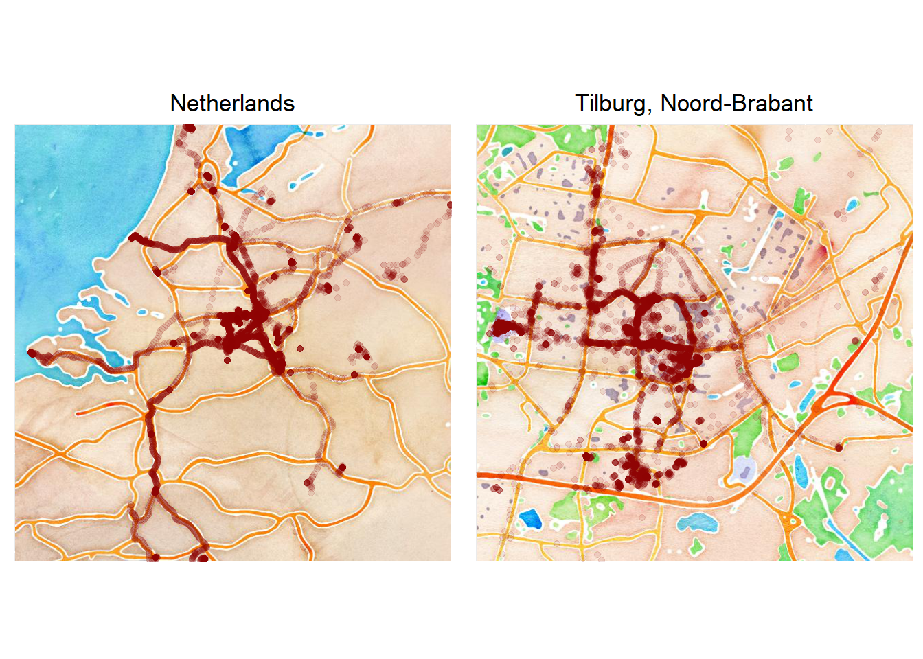

Interactive Visualisation

Below you can find an interactive map of my location. Scroll closer to enhance the clusters or heatmap and find out where I’ve been. It even shows where I went on holidays during this year!

## Create interactive Leaflet Map
Int_Map <- Locations_Aantal %>% 
  leaflet %>% 
  addProviderTiles(providers$OpenStreetMap) %>% 
  setView(lng = 5.0919143, lat = 51.560596, zoom = 5) %>% 
  addTiles() %>% 
  addMarkers(~lon, ~lat,  clusterOptions = markerClusterOptions(),
             group = "Cluster") %>%
  addHeatmap(lng = ~lon, lat = ~lat, intensity = ~Aantal,
             blur = 20, max = 0.05, radius = 15,
             group = "Heatmap") %>%
  addLayersControl(
        overlayGroups=c("Cluster", "Heatmap"),
        options=layersControlOptions(collapsed=FALSE)) %>%
    hideGroup(c("Heatmap"))